Enhanced Cell Tracking Analysis

Features in ModFit LT and WinList provide unparalleled capabilities to analyze cell proliferation.

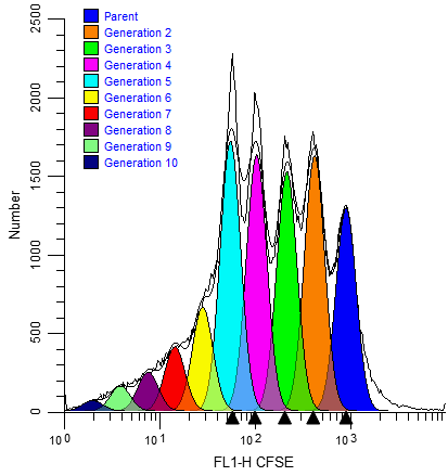
ModFit LT performs sophisticated least squares analysis in just a few clicks of a mouse and reveals the secrets of the proliferation data: proliferation index, non-proliferative fraction, and precursor frequency, and fractions for each proliferating generation. The proliferation results can be exported so that other applications can extend the analysis.

Enter WinList. NStat regions can import the proliferation results from ModFit LT, and then partition the generations according to the proliferation analysis. This enhancement sets the stage for exciting new analysis capabilities.

This tutorial will explore these new features to examine a CFSE-stained sample containing several other markers.

The big picture

From the Cell Tracking Wizard in ModFit LT...

$image\epa_ltmodel.jpg$

... into WinList for exciting, new explorations of proliferation.

$image\epa_wl1.jpg$ $image\epa_wl2.jpg$

Getting started

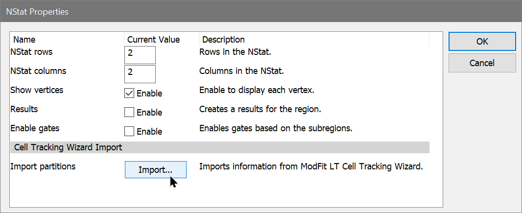
To start, we will use the Cell Tracking Wizard in ModFit LT and export its results. Then, you will set up WinList to import those results into an NStat region.

You will need both ModFit LT and WinList for this tutorial. WinList must be version 9.0 or greater.

Launch WinList and pass through the opening dialogs.
Launch ModFit LT and pass through the opening dialogs.
Using ModFit LT's Open FCS command, navigate to the Samples folder located in the WinList application folder. Select "CFSE sample.fcs" and click Open. Note, the dialog may look different than the one shown below, depending on the version of ModFit LT you are using.

$image\epa_ltparam.jpg$

Choose "FL1-H-CFSE" as the analysis parameter.
Next, right-click on the histogram and choose Edit X Parameter. Choose Log for the Transform and click OK.

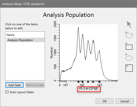
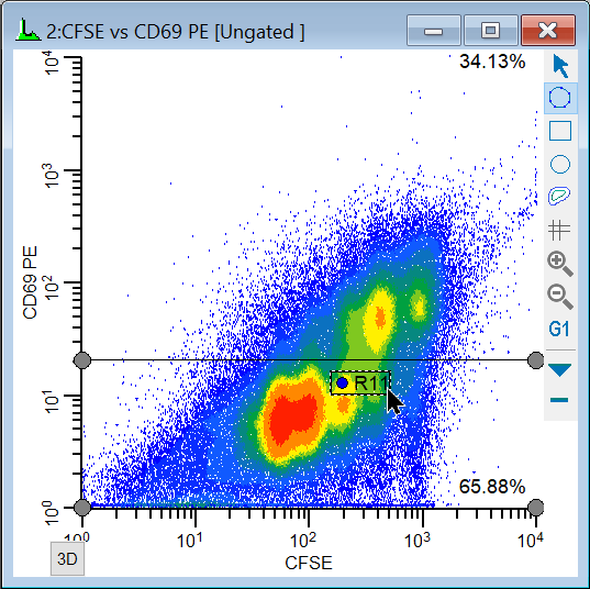
The axis now displays the Log transform. We don't need to create any gates - we'll do that later in WinList.

Click OK.
On ModFit LT's home tab choose Cell Track Wizard.
In the Cell Tracking Wizard dialog, click the Generations tab and choose the "Floating" model option from the drop-down list.
Click the Other tab, and enable Export partition table and Prompt for file name checkboxes. These options will cause the program to create the export file after analysis and allow you to enter a name for the export file.

$image\epa_ltexport.jpg$

Finally, click the Analyze button to perform the analysis.
When the analysis is complete, the Choose Location to Save Partitions dialog will be displayed. You can save the file to any location. For this tutorial, save the export file to the desktop so that it's easy to find later.

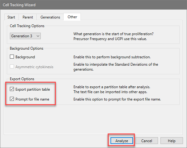
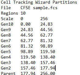
When you choose the Export option for the Cell Tracking Wizard, the program determines the boundaries between adjacent generations and writes that information to the export file. The boundaries are the points of intersection between the Gaussian components in the model.

$image\epa_ltexporttext.jpg$

Setting up WinList

Activate WinList and click the Open FCS button on the ribbon bar.
Navigate to the Samples folder located in the WinList application folder. Select the "CFSE sample.fcs" file and click Open.
In the Create Histograms dialog, select CFSE in the X Axis list and CD69 PE in the Y Axis list. Click Add to List two times. This will create two copies of CFSE vs. CD69 PE. Click OK to close the dialog.

$image\epa_wlhistsel.jpg$

You can change the graphical display for the histograms you've just created. Right click on the histogram and choose Graphics. Try out the different display options to see what you like best..

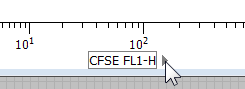
For this analysis we need to use a standard Log transform for the X and Y axis, not HyperLog. The exported information from ModFit LT is in Log units.

Move the mouse over the CFSE label on the X-axis and click the small triangle that appears. Select Log from the list of transformations. Repeat this for the CD69 Y-axis.

Click on the title bar of the first dot plot to activate it. Click the NStat region tool in the histogram toolbar.
In the NStat Properties dialog, click the Import button.

$image\epa_wlimport1.jpg$

Navigate to the Desktop folder and select CellTrackingWizardPartitions.txt and click Open.
Edit the NStat rows to 1 and check the Show Vertices, Results, and Enable gates checkboxes. The number of columns should already be 10 from the Import. Click OK.

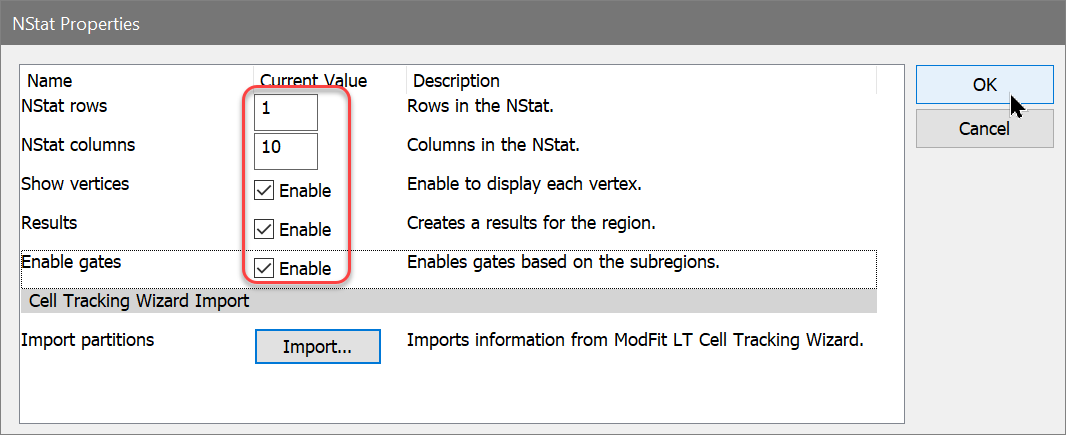
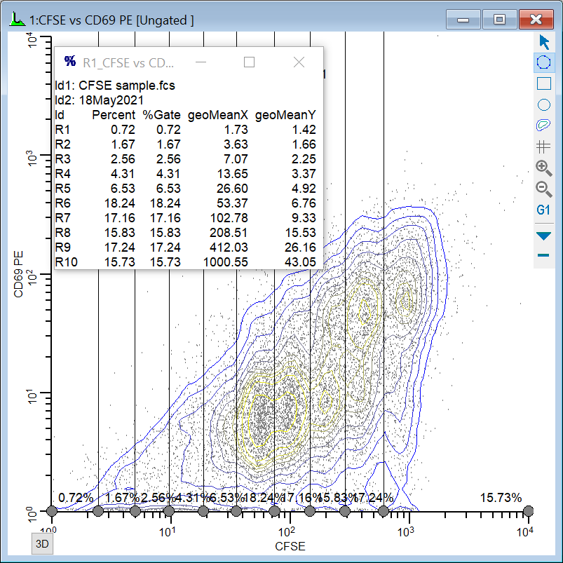
WinList creates the NStat partitions using the imported Cell Tracking information and displays a results window with statistics.

Isolating the generations

At this point, you have completed the basic import process. Let's extend the WinList analysis to explore other markers as a function of the proliferation analysis.

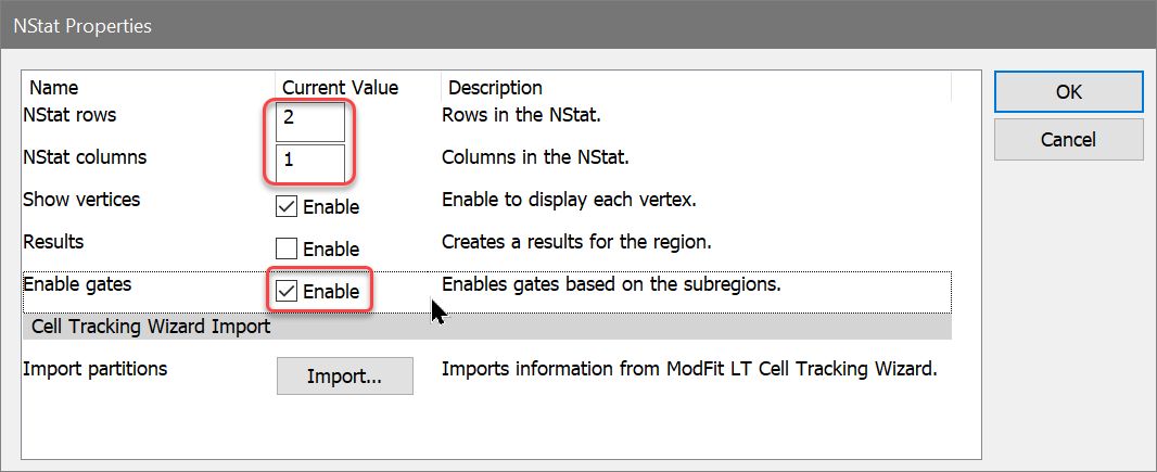
Click the title bar of the second histogram, and click the NStat region tool button to create another NStat. For this one, set NStat rows to 2 and NStat columns to 1. Check the Enable gates option and uncheck other options. Click OK.

Now, one of the histograms contains an NStat that shows the proliferation partitions, and the other histogram has an NStat that will allow us to define the CD69 negatives and positives.

Drag the region by the label to adjust the second NStat so that it approximately divides the two major populations in the second histogram, as shown.

You can change the graphics for any histogram by choosing Graphics from the right-click context menu for a histogram.

$image\epa_nstatpositions.jpg$

To analyze and visualize the generations better, we will create a calculated parameter using the FCOM function. This function creates a new parameter that will allow us to look at each population independently. It uses gates as input, and we'll use the gates from the NStat regions we just created.

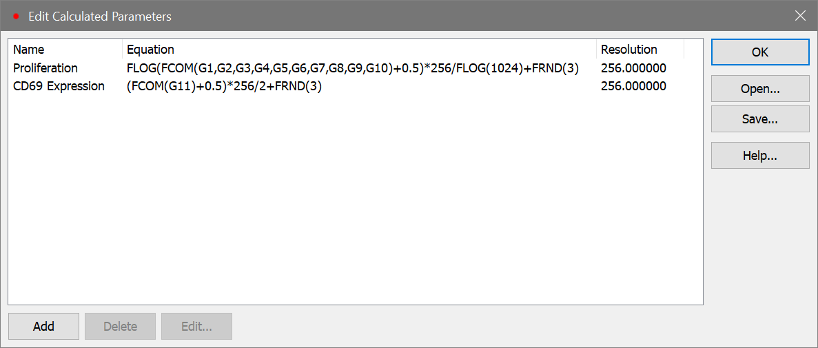
Let's create a few FCOM calculated parameters to help isolate the generations.

Click the Add Parameter button on the main ribbon bar. Alternatively, you can right-click in the data source and choose Add Parameter from the context menu.

Click the Add button in the Edit Calculated Parameters dialog.
Type Proliferation in the Name edit box. Type or copy this expression into the Equation edit box, and then click OK.

FLOG(FCOM(G1,G2,G3,G4,G5,G6,G7,G8,G9,G10)+0.5)*256/FLOG(1024)+FRND(3)

This expression deserves some explanation. Let's break it apart, starting with the FCOM portion. FCOM is a "gate combination" function. It takes any number of gates as arguments; the result of the equation depends on how many gates are in the expression. With a single gate, there are 2 possible event classifications: an event is "in" or "not in" the gate. With two gates, there are 4 possible event classifications. With the ten gates in our expression, FCOM can produce 1024 different event states.

However, since these gates do not overlap at all, most of the 1024 possible states have no events in them. In fact, the only states that contain events are the 10 single-positive event states, resulting in values of 1, 2, 4, 8, 16, 32, 64, 128, 256, and 512. If we plotted the result of the FCOM function as a histogram, we would see 10 spikes of events, and the spikes would be exponentially spaced.

Our goal is to see these 10 spikes evenly spaced across the histogram. This is where the FLOG function comes in. By taking the log of the FCOM output and scaling it by 1024, we redistribute the 10 FCOM values evenly across 256 channels. The final portion of the expression, "+FRND(3)", changes the spikes of events into Gaussian distributions so that they can be better visualized.

Take a look at the WinList reference sections on Add Parameters and FCOM for details on the complete set of WinList functions.

Once again, click the Add button in the Edit Calculated Parameters dialog.
Type CD69 Expression in the Name edit box. Type or copy this expression, and click OK.

(FCOM(G11)+0.5)*256/2+FRND(3)

$image\epa_addparam.jpg$

Click OK.

CD69 expression as a function of proliferation

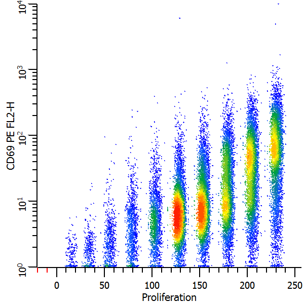
We're now ready to explore this data file in really interesting ways. Wouldn't it be nice to see CD69 as it relates to proliferation, viewing each generation as a discrete cluster? Could we quantify the CD69 expression of CD69-positive cells for each generation? Yes and yes.

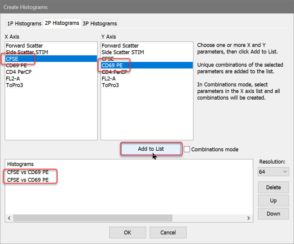
From the Insert tab on the ribbon bar, click the Density plot. This creates a Density plot in a default location on the data source. Click the X Axis label and choose Proliferation. Click the Y Axis label and choose CD69 PE.

Let's create another histogram to isolate the CD69 positives and negatives.

Right-click on the histogram that we just created and choose Clone from the context menu. A duplicate copy of the histogram is created.
Change the Y Axis to show CD69 Expression.

$image\epa_graph1.jpg$

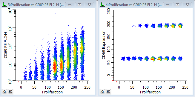
In the graphics we can see the generations separated into discrete populations along the X-axis. That's the first FCOM function we created. The Parent generation has the highest intensity.

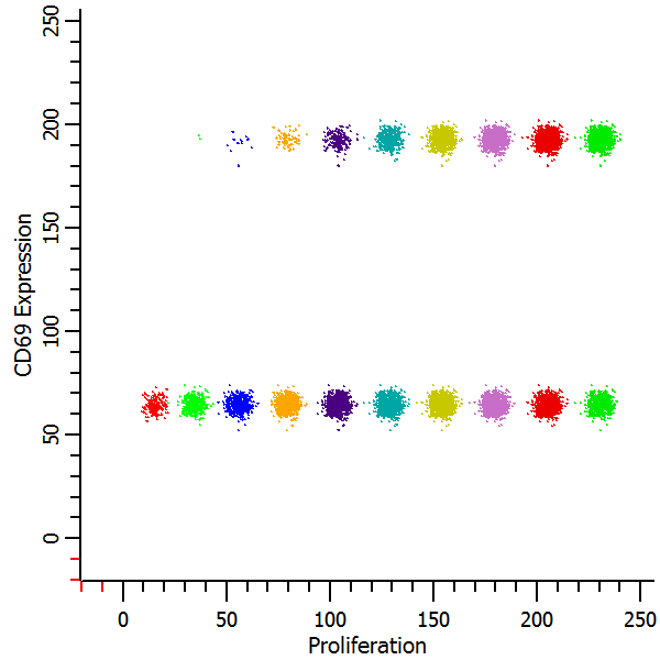
The Y-axis shows the continuous CD69 parameter in the histogram on the left. We can see that the parent generation had the greatest expression of CD69, with diminishing expression for each subsequent daughter generation. In the second plot. the CD69 positives and negatives are distinctly separated using the CD69 Expression FCOM parameter that we created. This makes it very easy to get statistics on the "CD69-activated" cells for each generation by simply creating regions on the subsets.

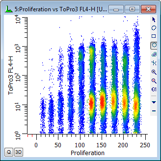
You can, of course, explore how other parameters relate to cell proliferation. Simply create additional histogram to display the parameter combinations you are interested in.

$image\epa_graph3.jpg$

Making life easier

You have done the real work in setting things up with this tutorial. If you save this setup as a WinList protocol or protocol bundle, the calculated FCOM parameters, NStat regions, and selected histogram can be recalled very easily from disk.

When you analyze new data files with ModFit LT's Cell Tracking Wizard, you can export new partition files. Then, open the same data file into your WinList protocol and import the partitions into the NStat region as we have demonstrated in this tutorial. All of the calculated parameters will update based on the new data and partitions.