Research
and Compliance Mode note:
In RUO mode, all users can perform these tasks.
In Compliance mode, only ModFitAdmins
have permission to perform them.
This section describes how to configure Auto Analysis to work with your data files. Three configuration dialogs are used to set up the program for Auto Analysis: Peak Finder Settings, Auto Analysis Settings, and Options and Configuration dialogs. By modifying the content of these three dialogs, you can optimize Auto Analysis to handle your data sets.
There are two major benefits to configuring the Auto Analysis system correctly. First, it will reduce the amount of time you have to spend analyzing each file. Of equal importance, you will increase user-to-user consistency of analysis results. The time you spend configuring the system can save analysis time in very few analyses.
Prerequisites
In order to complete this process, you need a data set of twenty or more data files of the same cell type that have been acquired according to the same protocol. Your protocol for sample preparation, staining, and acquisition should be well defined and strictly followed. Since different types of samples may have different characteristics and preparation procedures, you may need to configure the program differently for each type of sample you analyze.
Setting Options and Configuration
From the Options tab, choose Configuration. This will display a dialog containing a number of configuration settings. Most of these settings do not need to be changed from the program default settings.
One set of values you may need to adjust is found under the AutoLinearity section. The Low and High linearity values define the range over which the program can adjust the linearity during AutoLinearity adjustments when the AutoLinearity option is enabled. You should enter the acceptable range for G2/G1 ratios for your data set.
Review other settings in this dialog. For details on each setting, see Options and Configuration.
Make any adjustments required to the values. You may want to save these settings to a file that can be manually loaded back into the program. To do this, use the Save button at the bottom of the list in the dialog. When you need to re-open the saved settings, use the Open button. This also allows you to transfer settings from one computer to another.
Click OK to close the dialog and accept the changes you have made.
Reviewing a Data Set for Important Peaks
Next, the peak finder needs to be tested for your data set.
Click the Open FCS button on the Home tab. Navigate to the location of your data set and select twenty or more of the files to be analyzed. Click the Open button.
The program will open the first file in the set. If the file is a listmode file, you will need to select the parameter to analyze.
There are two things to notice at this point. At the bottom of the application window, the program now displays a batch navigation toolbar. We will use this to review the data set. Secondly, the first histogram has one or more peaks identified with black triangles along the x-axis. These are the peaks that the program's Peak Finder has identified. When the program is correctly configured for your data set, it will identify the vast majority of the internal standards and G1 peaks for cell cycles in your data set. It will also identify many of the well-defined G2M peaks, but these are not as critical as the G1 peaks. It should not identify many false peaks, that is, portions of the histogram that you do not consider to be real peaks.
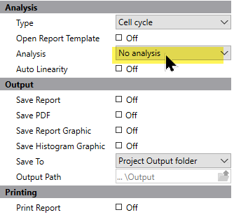
To review the data set, we need to tell the program what to do as we navigate through the batch of files. Click the left-most button on the batch control toolbar to display the properties for processing files.
Set the options as follows: No analysis and do not save or print reports, do not prompt for database or files. This tells the program that all we want to do is open the data files as we navigate through the batch.
Now, here is the process for peak finder review. For each file in the batch, record whether the program has identified all of the internal standards and the G1 peaks for each cell cycle. If the program misses an important peak, note the locations of peaks omitted. The major reasons peaks are missed are that they are too small, too wide, or they do not represent a normal, Gaussian distribution. All of these parameters can be adjusted in the program's peak finder. Also note the locations for any false peaks. For missing peaks and false peaks, try to note the characteristics of the peak, e.g. short, wide, shoulder.
Make notations for the files, and then click the "Next" button on the batch toolbar.

Repeat this process for each file in the data set.
Configuring Peak Finder Settings
Review the notations you made for the data set. If the program correctly identified 95% or more of the peaks in your test data set, you probably do not need to make any adjustments. If the Peak Finder did not perform as well as it should, here is how to make adjustments to the settings.
Hopefully, there are some common characteristics to the files that caused problems for the Peak Finder.
Use the batch navigation buttons on the batch toolbar to re-open a histogram that is representative of the mistakes the Peak Finder made.
Next, choose Peak Finder from the Options tab. The Edit Properties for Peak Finder settings dialog is displayed.
Click the Show button at the top of the list of options. This will display a dialog that allows you to see the current histogram, and to understand the characteristics of each peak.
As you move your mouse over the histogram, vertical lines will be displayed showing the boundaries for a peak that the program found. The lower portion of the dialog shows a number of peak filters, as well as the statistics for the peak your mouse is over.
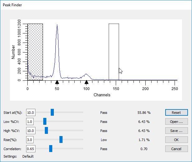
Example of Peak Finder with a "missing peak"
Move the mouse over a peak that the program did not identify. Look at the lower portion of the dialog for one or more of the settings that do not show the word "Pass". Adjust the sliders for the failing settings until all of the settings show "Pass" for the peak.
If no vertical lines appear for a peak, the peak does not qualify as a statistically valid peak. This kind of error cannot be corrected in the Peak Finder.
As you make adjustments, sweep your mouse across the histogram to review the status for all of the peaks. If you find that false peaks now "pass", you may need to compromise on your adjustments. If, however, the false peaks are very small, the program may exclude them from Auto Analysis for not passing other thresholds, so you should not worry about them at this point.
Once you have made adjustments that satisfy the histogram, click OK to close the Peak Finder dialog and return to the Edit Properties for Peak Finder settings dialog. You may at this point choose to save these settings to a file using the Save button at the bottom of the list. Alternately, you may want to write down the new settings. Since this process is experimental and may require several iterations, it is good to keep track of each set of adjustments.
Click OK to close the dialog.
Now you need to try out the new settings on the data set again. Move to the first file in the batch. Make notations for missing peaks and false peaks, and then move to the next file.
Repeat this process of reviewing and adjusting until the Peak Finder is tuned for your data set.
Adjusting Auto Analysis Settings
The final phase in optimizing Auto Analysis for your data makes use of the Auto Analysis Settings dialog. This dialog controls how the program interprets the peaks in a histogram.
From the Options tab, click Auto Analysis. The Auto Analysis Settings dialog will be displayed.
The first three options are straightforward. We recommend that you enable AutoDebris and AutoAggregates, as these components are robust and automatic in the way they handle debris and aggregation in samples. The Apoptosis option should be disabled for Auto Analysis unless you have a series of files in which you want to model apoptosis as a Gaussian distribution below the first cycle's G1 peak.
For Linearity, either leave the value at 2.0 or enter the average G2/G1 ratio of a data set. The G2/G1 ratio is easily computed by dividing the mean channel of a G2 peak by the mean channel of the G1 peak of the same cycle. Typical ranges are 1.95 to 2.0.
In the Standards and Reference section, enter the number of internal standards your samples contain. If you have internal standards, you should click the Edit button to set the properties of the standards. The most important property to set for each standard is its expected channel position. By entering an expected position, the program can make better decisions about when peaks shift and where the first cycle begins.
If you want to make use of an external reference standard for determining the location of the Diploid population, you should enter its channel location. This is only required if you want to base the Diploid position on the external reference.
The Ploidy Determination section provides a number of interesting possibilities for assigning ploidy labels to peaks. We will examine these in detail.
First, the Maximum cell cycles entry can in most cases be set to Unlimited. However, if you want to restrict Auto Analysis to creating models with a limited number of cell cycles, select the number of cycles in this drop down listbox.
The Diploid determination list presents 4 options for determining which cycle is labeled "Diploid". The first option, "First cycle is Diploid", simply assumes that the first peak, after any internal standards and apoptosis, is the Diploid G1 peak. This option should be used for paraffin samples. When you use this option, you do not need to enter a value in the related field, Diploid-to-Standard ratio.
You can also choose to base the Diploid cycle decision on the position of one of the internal standards or an external reference channel position. In these cases, you need to enter the expected Diploid-to-Standard ratio. For example, if your 2nd internal standard appears at channel 40 and you expect the Diploid G1 to be at channel 50, you can choose "Based on Standard2" for Diploid determination and enter 1.25 for the Diploid-to-Standard ratio. (Note: The value 1.25 in this example is for PI-stained trout red blood cells in relation to PI-stained human Diploid cells. For DAPI staining or other internal standard cells, the ratio will be other values.)
The G1 threshold field determines how big a peak has to be in order for it to be called a G1 peak. This is a relative height after adjustment for aggregates. In essence, it acts like another filter in the Peak Finder specifically for G1 peaks. If you have a number of small peaks that Auto Analysis is calling G1 peaks and you do not want them classified that way, increase the G1 threshold about 2 or 3 units at a time until they are not longer considered G1 peaks.
The Peak Location Range field determines how much of a shift from the expected locations you will allow. For example, if the value is set for 10 (percent) and the Diploid is expected to occur at channel 50, the program will look for a peak between channel 45 and 55. Generally, values between 5 and 10 are best for this field.
The S-Phase group does not require adjustments for most users. The settings are based on industry-standard recommendations and practices, so if you change these settings, it will be difficult or impossible to compare results in your lab with results of other labs.
The Tetraploid group allows you to set the threshold at which the program will call a peak a Tetraploid G1 instead of a Diploid G2M. Recommended values range from 15 to 25, and you may need to experiment with these values on your data set.
When you finish making your first adjustments to the settings, use the Save button to save the settings to a file on disk. As with other configuration dialogs, you may need to go through several iterations before you find the best settings for your data set.
Choose OK to close the dialog.
Testing the Auto Analysis settings
At this point, you are ready to test the full system.
Change the file processing settings to Auto-analyze each data file that you open.
Click the "go to first" button on the batch control toolbar. The first file will be opened and an Auto Analysis will be performed. Make a notation to indicate whether the program correctly analyzed the data. Pay particular attention to the ploidy classifications for each cycle and the graphical representation of the fit.
Advance to the next file. After the program auto-analyzes the file, make notations about the success or failure of the program. Repeat this process for the entire data set.
After all files have been processed with Auto Analysis, review your notations. The goal is to have the program work automatically for greater than 95% of the files. If you need to make additional adjustments, repeat the process of reviewing and adjusting until you achieve the best results.
When you have the settings that work best, display the Auto Analysis Settings dialog once again. Save the settings to a file using the Save button. Click OK to close the dialog.
Summary
The process of tuning Auto Analysis for your own data sets involves three dialog boxes: Options and Configuration, Peak Finder Settings, and Auto Analysis Settings. After setting up configuration options, an iterative process is used to find the best Peak Finder Settings for a data set. As the final step, a similar iterative process is used to tune the Auto Analysis Settings to a data set.
Use a data set of samples from the same cell or tissue type. As you perform this process for a data set, save your settings for each dialog box so that they can be reloaded at any time.
You should perform this process for different sample types if the preparation process or the data files themselves have difference characteristics from the data set initially used to optimize Auto Analysis.
You will always find some files in a data set that are unusual when compared with the rest. Do not try to optimize Auto Analysis for unusual data, or you will find that it fails more often than it works. Instead, base your decisions on the typical data in a data set, and you will find the system has a much higher success rate.
See also: